Consumption effects of job loss expectations: new evidence for the euro area

expectations: new evidence for the euro area
Disclaimer: This paper should not be reported as representing the views of the European Central Bank (ECB). The views expressed are those of the authors and do not necessarily reflect those of the ECB.
Abstract
Probabilistic job loss expectations elicited in the Consumer Expectations Survey have predictive power for future job loss. We find that an unexpected job loss leads to a negative consumption response, while this effect is muted for workers with ex-ante job loss expectations - consistent with the Permanent Income Hypothesis. The negative consumption response to an unexpected job loss is stronger for workers who have worse perceptions of the local labour market, are older or have lower levels of liquid wealth. This supports the notion that the persistence of the unemployment shock is an important factor of the consumption response to a job loss. At the same time, we do not find a positive consumption response of workers who unexpectedly retain their job. These heterogeneous results have important implications for the expected impact on consumption of job protection measures such as job retention schemes.
JEL classification: D12, D84, J63
Keywords: job loss expectations, consumption, ECB Consumer Expectations Survey (CES),
Permanent Income Hypothesis (PIH)
Non-technical summary
Job loss is a severe event for individuals and households. It affects income, savings and consumption opportunities, sometimes for a prolonged period of time. Households often reduce their consumption of non-necessities or deplete their savings in order to cushion the impact of the reduced income. This affects aggregate demand and prices in an economy. Hence, it is of crucial importance for central banks to understand the economic reaction of households to a job loss.
At the same time, a job loss is often not completely unexpected. Workers sometimes know well in advance that they might experience a displacement in the near future. This might for instance be the case if they were notified by their firm in advance or because they are aware of a challenging competitive or business situation of their firm. Accordingly, previous economic literature has shown that households adjust their consumption and savings behaviour already before the actual time of the job loss.
In this paper, we empirically test how households adjust their consumption to an unexpected job loss and compare it to the reaction to an expected one. To this aim, we use a recently developed survey by the European Central Bank (ECB) that asks workers across a set of euro area countries (Belgium, France, Germany, Italy, Spain and the Netherlands) about their current labour market situation and expectations for the coming quarter. The ECB Consumer Expectations Survey (CES) also contains information on the latest consumption of households.
This allows us to combine the information of job loss, job loss expectations and consumption.
We first show that job loss expectations are consistent with expected income growth and have predictive power for actual job loss. However, workers overestimate the chance to lose their job. Across all countries and income groups, job loss expectations exceed actual job loss realisation rates. At the same time, workers have some knowledge of their own job loss probability. The higher workers’ job loss expectations, the higher the chance that they will actually lose their job in the coming months. This means that while job loss expectations elicited from surveys might not be accurate, they still contain valuable information for central banks and other policy makers about future labour market conditions.
In addition, we show that households’ consumption reacts to a job loss in line with theoretical predictions. It is unanticipated income changes rather than anticipated ones that determine the adjustment of consumption behaviour. While for some individuals job loss is fully expected, for many others it occurs as a surprise. We explore errors in individuals expectations about their job loss and show that workers who fully anticipated their job loss do not adjust their household consumption following the displacement. Previous work has shown that they instead adjust their spending already at the time they learn about their upcoming job loss. Workers who did not anticipate their job loss, however, reduce their consumption following their displacement. We show that this reaction is stronger for groups who perceive the labour market situation to be worse, older workers and workers with a lower level of liquid financial means. These workers are more likely to reduce their spending more extensively as they expect their job loss to be more persistent or are more dependent on their income to cover their level of consumption.
Overall, our work shows that expectations elicited from surveys contain valuable information for policy makers. They allow to better understand economic behaviour of households around the time they experience a job loss or labour market uncertainty. This helps to improve the interpretation and timing of demand and price fluctuations during recessions as well as the targeting and effectiveness of policy measures such as job retention schemes.
1 Introduction
Individuals have information about their future labour market status that is unavailable to the econometrician and is usually a part of the unexplained heterogeneity. Starting with Manski and Straub (2000), it has repeatedly been shown that elicited survey expectations have consistent explanatory value for future realisations of individuals’ labour market status and therefore can reduce this unexplained component. However, there is little evidence on how this individual information shapes economic behaviour at the time it becomes available and realises.
In this paper we show that job loss expectations affect consumption behaviour in a way that is consistent with the predictions of the permanent income hypothesis (PIH). The PIH states that consumption should only react to a job loss to the extent that it is inconsistent with prior expectations. Thus, there should be an immediate reaction of consumption at the moment the job loss becomes known to the worker and consumption should not react at the time of displacement if it was fully anticipated.
To test this prediction, we use the recently developed Consumer Expectations Survey (CES) of the European Central Bank (ECB), which collects data on expectations and consumption, and explore errors in workers’ job loss expectations. While workers are on average good predictors of their own job loss, some individuals become displaced despite low job loss expectations and others remain employed despite high job loss expectations. We exploit this variation in expectation errors to assess consistency of consumption behaviour with the predictions of the PIH following an unexpected labour market outcome. In this approach, workers who are dismissed without fully expecting it make a negative expectation error and workers who retain their jobs despite having attributed some probability to job loss make a positive error (as in Stephens 2004). The PIH predicts that only workers with such erroneous expectations should adjust their consumption in line with their unanticipated employment status.
First, we show that workers are on average good predictors of their individual labour market outcomes. While individuals on average overpredict their own job loss probability, their expectations and realisations are systematically positively correlated. In a Probit regression design following similar work for instance by Dickerson and Green (2012) or Pettinicchi and Vellekoop (2019), we find that workers who have 10pp higher job loss expectations have an about 0.6pp higher probability of job loss in the following three months. This is in line with previous findings and confirms the predictive value of survey-based job loss expectations.
Second, we show that errors in assessing one’s future labour market outcomes can have an impact on consumption behaviour. Individuals who lose their job unexpectedly depict a significant negative consumption response. However, this response is muted if individuals had ex-ante expectations of job loss. These results are in line with the prediction of the PIH but at odds with previous findings by Stephens (2004) who found no consumption effect of erroneous expectations beyond a consumption effect of anticipated displacement - contradicting the theoretical predictions. However, similar to his findings we do not find a symmetric positive response of individuals who unexpectedly remain employed. This means that while job loss expectations seem to matter much less in case an expected displacement did not materialise, they have a decisive impact on consumption developments following a displacement.
We further investigate these results exploiting the drivers of the effect by assessing its heterogeneity across various subgroups. The CES data allow us to analyse a variety of factors as well as potential explanations for the observed expectations and consumption patterns. We show that the sensitivity of consumption with respect to job loss expectations is larger for workers who perceive the unemployment rates to be above the median perceptions in their country. This is also in line with the PIH that predicts the consumption drop to be proportional to the expected reemployment probability of individuals. For workers with worse perceptions of the labour market, the expected persistence of a job loss is larger. This implies a stronger consumption response to a displacement relative to regions with more benign labour market conditions. These results are confirmed by the observation that also older workers show a stronger sensitivity of their consumption to their ex-ante expectations.
Finally, we are able to show that workers with a lower level of liquid wealth ("hand-to-mouth") have a stronger consumption response to a displacement shock than wealthier individuals. Households with a higher level of liquid assets are better able to smooth their consumption profile and depend to a lower degree on their current labour market income. Hence, we show that the standard predictions of the PIH hold for displaced workers in the euro area.
With our analysis we contribute to the empirical literature on how expectations affect economic behaviour prior to as well as conditional on their realisation. Such expectations are key for economic models of consumer decision-making, such as life-cycle models and models of precautionary savings (Dominitz 2001). Elicitation of expectations from surveys, in particular those with probabilistic content, have been shown to be consistent and credible, and hence suitable for informing structural economic models (e.g. Dominitz and Manski 1997, Dominitz 2001, Manski 2004). We confirm prior findings that job loss expectations are consistent with other survey-based measures. The multi-country perspective of the CES and the large sample size allow us to assess the heterogeneous impact of job loss expectations in a unique setting. Using this new set of data with quarterly job loss expectations, we show that such short-term job loss expectations have predictive power for job loss realisations in line with similar measures that have been used in previous work. Therefore, we are able to add to the discussion on the importance of expectations management and public communication of fiscal policies in limiting expectationdriven pro-cyclicality (see also Enders et al. (2022) for the effects of firm-side expectation errors).
We also contribute to the assessment of the empirical predictions of the PIH. Earnings of displaced workers have been shown to decline substantially and persistently after displacement (e.g. Jacobson et al. 1993) with consequences for consumption behaviour (see e.g. Stephens (2001) or Meghir and Pistaferri (2011) for an overview). Prior findings confirmed the PIH hypothesis that consumption reacts stronger to unexpected changes in income expectations than to expected ones (e.g. Penrose and La Cava 2021). Stephens (2004) shows that this only holds for negative shocks and can mostly be explained by the income effect of displacement rather than erroneous expectations. Contrary to his findings, we find no significant impact of displacement if it is fully anticipated - in line with the predictions of the PIH. Instead, consumption only drops if the displacement was at least partially unanticipated.
The paper is structured as follows: First, we introduce the previous literature on job loss expectations and evidence on the PIH. Afterwards, we give an overview of our job loss expectation data in the CES and show that they are consistent across survey replies and predictive of actual job loss. Then we explain our empirical approach closely following the standard specification of the PIH. Using this specification as a benchmark, we finally discuss the impact of expectations on different measures of consumption and analyse the predicted heterogeneity across individuals.
We conclude with a discussion of policy consequences of our results.
2 Literature Review
In the empirical literature, the role of individual expectations in shaping consumer behaviour has been investigated even before surveys eliciting such expectations became available. However, for a long time, expectations could only be recovered indirectly - for instance, income expectations were inferred from income realisations (e.g. Dominitz 2001). Since then, the analysis has strongly benefited from the introduction of surveys asking households directly about their expectations, especially those using cardinal scales and probability values. The latter’s predictive performance has been shown to be superior to that of the surveys using only qualitative replies and ordinal scales (Dickerson and Green 2012).
Subjective probabilities of job loss have been found to be positively and significantly correlated with subsequent realisations of job loss, usually defined as the share of workers who actually lost their job (Stephens 2004, Campbell et al. 2007, Dickerson and Green 2012, Pettinicchi and Vellekoop 2019, Hendren 2017, Mueller and Spinnewijn 2021). This relationship holds true even after controlling for social characteristics such as age, education and job tenure, which implies that expectations reflect unobserved characteristics or own superior information of individuals, correlated with their labour market outcomes. However, there is a lack of agreement in the literature about the strength and magnitude of the relationship. For instance, McGuinness et al. (2014) only find a weak relationship between job expectations and subsequent transitions to unemployment or inactivity. Regarding the magnitude, elasticity estimates range between 0.10 - 0.12 (e.g. Dickerson and Green 2012) and 0.89 (e.g., Pettinicchi and Vellekoop 2019). In the former case, this means that 1 percentage point increase in the expected probability of job loss is associated with an increase of about 0.1 percentage points in the probability of actually losing the job.
Most studies document that workers tend to overestimate their probability of job loss, i.e. the subjective job loss probability tends to be higher than the realised probability measured as the share of workers who lost their job (e.g. Dickerson and Green 2012 for the US, Penrose and La Cava 2021 for Australia)[1]. The relationship between expected and actual probability of job loss is also sometimes found to be nonlinear, being weaker for higher values of job loss expectations (e.g. Penrose and La Cava 2021). On the other hand, there is also evidence that respondents who report a zero perceived probability of job loss underestimate the probability to some extent (e.g. Dickerson and Green 2012).
While the predictive property of job loss expectations for future labour market transitions is important on its own, these expectations also play a role for consumption behaviour. Job insecurity is an important source of income insecurity for households, which leads to precautionary savings in the standard life-cycle model of consumption (e.g. Benito 2006).
Workers facing a decline in household income, in accordance with the PIH, can be expected to adjust their consumption if they regard the potential income change as permanent or long-lasting (see, for instance, Hall and Mishkin 1982). Individual job loss expectations are indeed correlated with individual income expectations, as shown empirically by Dominitz (2001), also when controlling for a range of demographic characteristics and current income. Benito (2006) and Carroll and Dunn (1997) confirm an inverse relationship between job insecurity and household non-durable consumption. Moreover, the former study finds that the relationship remains significant even controlling separately for income expectations, concluding that unemployment expectations are at least as important as income expectations for explaining non-durable consumption. Consumption of durable goods is generally more pro-cyclical and can be expected to be stronger affected by income changes than non-durable consumption. Quality as well as availability concerns make these data hard to use in empirical analysis. Therefore, most available studies focus on food consumption. Among the few studies looking at durable consumption, Pettinicchi and Vellekoop (2019) establish a weak negative relationship between expectations for job loss and purchase of new cars. They also document that respondents with higher probability of job loss seem to have more precautionary savings.
It has been amply described that households decrease consumption as a result of an actual job loss (Hendren 2017, Christelis et al. 2015, Browning and Crossley 2001). Gruber (1997) estimates that the consumption decline at job loss amounts to 20 percent. In order to capture correctly the consumption impact of a job loss, it is important to differentiate unexpected job losses from job losses which have been predicted. In line with the PIH, household consumption should not react to a displacement if they have perfectly foreseen it (e.g. Penrose and La Cava 2021), and the larger the surprise from the job loss, the larger the current income shock should be. As Campos and Reggio (2015) argues, an unexpected job loss impacts consumption via two channels: through current income and through expected future income if the job loss is expected to lead to persistent earnings loss. They find that the crucial impact comes from innovations to future income growth, while the impact from current income innovations is limited.
In contrast with the theoretical PIH predictions, the empirical evidence regarding the impact of unanticipated job losses or expectation errors is not conclusive. While households indeed seem to react to unexpected job loss or change in their income (e.g. Penrose and La Cava 2021), the role of anticipated changes is not zero as theoretically predicted. Stephens (2004) does not find evidence that the previous expectations of households can reduce the impact of job loss on consumption. The quantitative impact of displacement itself can be larger than that of a (partial) displacement surprise. Likewise, Penrose and La Cava (2021) using Australian data find that the degree of spending reduction at job loss is independent of whether the job loss was expected or not. Pettinicchi and Vellekoop (2019) find evidence of an asymmetric response of durable consumption, as only negative expectation errors (where respondents’ probability of a job loss was too low) are significant.
The magnitude of the consumption reduction at job loss also varies with some additional factors reflecting the resources available to the household to cushion the unemployment shock. Benito (2006) shows that the relationship between job loss probability and non-durable consumption is stronger for younger workers, those without non-labour income or who have been unemployed for a longer time. The elasticity is found to be higher for households with lower wealth (Browning and Crossley 2001), those who have accumulated higher debt (Carroll and Dunn 1997) or who face lower replacement rate of the unemployment insurance (Gruber 1997).
The current paper is also related to the literature on savings in the context of the validity of the PIH (Jappelli and Pistaferri 2000 or Christelis et al. 2020). In many empirical studies savings are derived as the difference between income and consumption. Hence, if the PIH holds, savings should respond to transitory but not to permanent shocks. However, most of the empirical evidence seems to point to the opposite. Pistaferri (2001), using income expectations and realisations to distinguish transitory from permanent income shocks, shows that the predictions of the PIH do not hold, as savings seem to react also to permanent income shocks.
3 Data
We use CES data from April 2020 to January 2023 for six euro area countries (Belgium, France, Germany, Italy, Netherlands, Spain).[2]The CES is a mixed-frequency panel survey that elicits a variety of individual expectations, behavioural and socioeconomic variables (see ECB (2021) and Georgarakos and Kenny (2022) for an overview).
The CES elicits job loss expectations of employed workers three months ahead with the question: "What do you think is the percent chance that you will lose your current job during the next 3 months?". Workers can answer any integer between 0 and 100 percent. This is the question we use to measure workers’ job loss expectations. The data do not allow to distinguish Figure 1: Distribution of job loss expectations
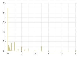
Note: Histogram of 3-month job loss expectations.
Source: CES data.
between voluntary and involuntary job loss. However, the survey explicitly asks for job "loss", which might indicate an involuntary action. In a robustness exercise, we also limit our analysis to workers whose job spell is followed by unemployment (with active job search). This indicates a continuing labour market attachment and hence a lower likelihood of having left one’s previous job voluntarily.
Empirically, job loss expectations are on average rather low, bunching at certain digits, and right skewed (see Figure 1 and Table 1), which is in line with other surveys eliciting job loss expectations, such as the US Health and Retirement Survey (HRS) used by Stephens (2004). The median respondent expects a 1% probability to lose her job in the next three months. More than 35% of all respondents even expect a 0% probability. Hence, most respondents have low expectations of job loss. However, average job loss expectations are above 10%. Among respondent with non-zero job loss expectations the average is even around 20% (see Figure 2). Hence, respondents for which a displacement is not completely implausible show a considerable variation of expectations.
Unlike previous literature that uses 12-month expectations, quarterly expectations allow us to analyse job loss expectations at a higher frequency and the shorter foresight period should improve the quality of replies. As the CES elicited 3- and 12-month expectations contemporaneously in five ad-hoc modules during 2020, we are able to show the high correlation of expectations with different frequencies. Figure 2 shows that 3-month expectations are rather stable over time and move in parallel to 12-month expectations. In addition, 12-month Table 1: Job loss expectations: 3 vs. 12 months ahead
mean | p10 | p35 | median | p65 | p90 | n | |
Job loss expectations | 0.109 | 0.00 | 0.00 | 0.01 | 0.05 | 0.40 | 90534 |
Job loss expectations (subsample) | 0.117 | 0.00 | 0.00 | 0.02 | 0.06 | 0.45 | 12394 |
Job loss expectations (12 months) | 0.139 | 0.00 | 0.00 | 0.05 | 0.10 | 0.50 | 12394 |
Absolute difference | 0.040 | 0.00 | 0.00 | 0.00 | 0.00 | 0.10 | 12394 |
Note: Distributions of 3-month job loss expectations (row 1), using the same sample as 12-month expectations (row 2) and 12-month expectations (row 3). The last row shows the distribution of the absolute difference between 12- and 3-month expectations.
Figure 2: Expected job loss probability
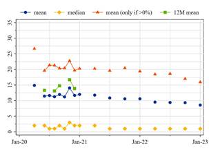
Note: The blue and yellow dots show mean and median of 3-month job loss expectations, respectively. The red dots shows the average for respondents with non-zero expectations. The green dots shows the average of 12month job loss expectations. Source: CES data.
expectations have a higher mean and median, but we find that two thirds of respondents answer exactly the same and 90% at most 10pp more (see Table 1). This is not only driven by double zero answers. Overall, 3-month expectations seem to be a valid measure of job loss expectations.
Most labour market variables and expectations are asked in the quarterly module of the CES. Therefore, we focus on a quarterly frequency in our analysis.[3]In addition, since individual income is only available from October 2020, all results using income data start only in that month. This also means that our data does not cover the beginning of the COVID pandemic that entailed large distortions on the labour market. On the contrary, it covers the recovery period after the unemployment rate in the euro area reached its peak in September 2020 with 8.6% before rapidly falling back below pre-crisis levels in the following months. Hence, we should not observe excessively many unexpected job losses that might translate into reductions Table 2: Descriptive statistics


Note: Average values of employed workers by job loss status in t + 1 weighted by population weights. The education level is aggregated into three categories low, medium, and high that represent below upper secondary, upper secondary and tertiary education, respectively. Job loss expectations range from zero to one. Standard deviations in brackets. Source: CES data.
of consumption. Instead, our estimates rather constitute a lower bound of the potential adverse impact of business cycle dynamics on consumption.
We define job loss of a worker as a dummy variable equal to one if a respondent is employed at t and either unemployed or inactive at t+3, where t is the month of the survey.[4]We focus on prime-aged respondents aged 25-59 to avoid any ambiguity in capturing retirement or education transitions instead of job loss. Overall, we observe more than 2,000 transitions out of employment in our data (see Table 2). Respondents who lose their job have more often a short tenure, a low education level and are slightly younger. They do also have higher job loss expectations (above 25%, in comparison to just 9% for those with no job loss) and therefore consistent expectations of their subsequent labour market status.
4 Consistency and predictive power of job loss expectations
Before analysing our main question of interest the relation between job loss expectations and consumption behaviour we want to assess the quality of the job loss expectations variable. To assess consistency, we analyse the relation between job loss expectations and measures of income in the survey. To assess predictability, we analyse how job loss expectations are correlated with actual job loss.
4.1 Consistency of job loss expectations
We assess consistency of job loss expectations as reported in the CES by relating them with replies to other questions about labour market outcomes. To this aim, we run a linear OLS regression of job loss expectations on different measures of income expectations that are available in the CES. The first two columns of Table 3 use ordinal income growth expectation.[5]In model (1) we quantify them as -1 if income is expected to decrease, +1 if income is expected to increase and 0 otherwise. For model (2) we further differentiate between strongly decreasing (-2) and strongly increasing (2) income expectations. Model (3) finally uses quantitative income growth expectations in percentage points.[6]After controlling for person, date, tenure and income fixed effects, we find a large R2 of around 0.4. This hints towards a strong co-movement of expected job and income loss.
Overall, job loss expectations seem to be consistently negatively correlated with different measures of expected income growth during the following year. This is consistent with a job loss and subsequent persistent income loss. Results from model (3), using a quantitative scale, show that an increase in job loss expectations of, for instance, 10pp is related to a 0.41pp lower expected household income growth. This is a considerable reduction relative to an average expected income growth of 1.14% and a median of zero. Thus, job loss expectations are likely to also have a bearing on consumption behaviour.
Table 3: Job loss and income expectations
(1) | (2) | (3) | |
Exp. income growth bracket | Exp. income growth bracket | Exp. income growth | |
Job loss expectations | -0.2036*** | -0.2841*** | -4.0966*** |
(0.0381) | (0.0522) | (0.6584) | |
Person FE | Yes | Yes | Yes |
Date FE | Yes | Yes | Yes |
Tenure bracket FE | Yes | Yes | Yes |
Income bracket FE | Yes | Yes | Yes |
N | 38688 | 38688 | 38688 |
Unique N | 7868 | 7868 | 7868 |
R2 | 0.40 | 0.40 | 0.48 |
Note: The dependent variable is bracketed 12-month income growth expectation in model (1) and (2) and absolute (non-bracketed) income growth expectations (in pp) in model (3). Robust standard errors clustered on individual level in parenthesis. Stars denote significance levels of two-sided t-tests. * p < 0.1, ** p < 0.05, *** p < 0.01
4.2 Predictive power of job loss expectations
We also assess if job loss expectations have predictive power with regards to actual displacement. As described above, we measure displacement as employed respondents who report to be unemployed or inactive in the following quarterly survey. As can be observed from Figure 3, displaced workers have on average a higher job loss expectation. Nearly 10% of respondents who are later displaced fully expected their displacement one quarter ahead. At the same time, a large share of job losses is unexpected. There is a considerable share of workers with zero or close to zero job loss expectations who still become unemployed or inactive three months later. In fact, 36% of all workers who lose their job report a less than 5% probability for this to happen (and 26% even exactly zero probability). Hence, there is a large variation in the predictive power of job loss expectations that we will exploit for our analysis.
Nevertheless, job loss expectations are on average overestimating actual job loss, which is also in line with the previous literature. This is the case for all income groups and the six countries in our sample. Figure 4 shows average expectations and realisations for respondents within each of ten income brackets separately for each country.[7]Workers in lower income groups tend to have higher job loss expectations. However, they are not necessarily more accurate. For most countries there is a strong positive correlation of job loss expectations and job loss Figure 3: Distribution of job loss expectations by displacement status
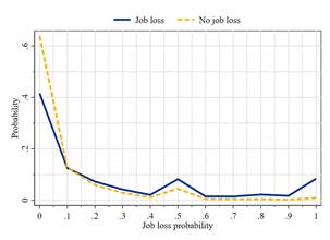
Note: The lines show the distribution of job loss expectations aggregated into 11 bins by displacement status in t +1. Source: CES data.
realisations across income groups.[8]However, the expectations all lie below the actual job loss probability within each group. Hence, despite the high share of workers with low or zero job loss expectations, the average job loss expectation lies above the realised value.
In order to establish the statistical relationship of job loss expectations with realisations, we run a Probit estimation following various previous approaches in the literature (see Section 2). To this aim, we regress displacement on previous job loss expectations while controlling for time and country effects as well as various socio-demographic characteristics that might affect this relationship (see Table 4).
We find that a one standard deviation (18.8pp) higher expectation is related to a 2.1pp higher job loss probability (average marginal effect). The relation is slightly lower at 1.56 when controlling for tenure, education level, gender, age group, partnership status and number of household members. Model 3 to 6 control in addition for individual income brackets. Since income data are only available from October 2020, we lose some observations for these regressions. While the relationship remains significant at the 1 percent level, the link seems to be weaker if we control for income brackets. Nevertheless, since income is an important component of job risk, model (3) is our preferred specification with a positive correlation of around 0.06 between job loss expectations and realised displacements.
Table 4: Job loss expectations and job loss realisations
(1) | (2) | (3) | (4) | (5) | |
E to Non-E | E to Non-E | E to Non-E | E to UE | E to Non-E until t+4 | |
Job loss expectations | 0.1133*** | 0.0829*** | 0.0633*** | 0.0261*** | 0.1321*** |
(0.0051) | (0.0048) | (0.0046) | (0.0021) | (0.0130) | |
Secondary | -0.0190*** | -0.0109* | -0.0001 | -0.0310 | |
(0.0055) | (0.0049) | (0.0023) | (0.0161) | ||
Tertiary | -0.0235*** | -0.0108* | -0.0015 | -0.0269 | |
(0.0051) | (0.0046) | (0.0021) | (0.0152) | ||
Female | 0.0076** | 0.0036 | -0.0004 | 0.0005 | |
(0.0024) | (0.0024) | (0.0012) | (0.0074) | ||
30-39 | -0.0034 | -0.0005 | 0.0016 | -0.0131 | |
(0.0050) | (0.0051) | (0.0019) | (0.0163) | ||
40-49 | -0.0153** | -0.0124* | -0.0010 | -0.0413* | |
(0.0050) | (0.0050) | (0.0019) | (0.0163) | ||
50-59 | -0.0054 | -0.0053 | 0.0019 | -0.0242 | |
(0.0052) | (0.0052) | (0.0021) | (0.0168) | ||
Partner in HH | 0.0004 | 0.0023 | 0.0007 | 0.0091 | |
(0.0029) | (0.0029) | (0.0013) | (0.0096) | ||
HH members | 0.0034** | 0.0020 | -0.0001 | 0.0060 | |
(0.0012) | (0.0012) | (0.0006) | (0.0041) | ||
Country FE | Yes | Yes | Yes | Yes | Yes |
Date FE | Yes | Yes | Yes | Yes | Yes |
Tenure bracket FE | No | Yes | Yes | Yes | Yes |
Income bracket FE | No | No | Yes | Yes | Yes |
N | 48816 | 48816 | 40813 | 40543 | 18335 |
Unique N | 11029 | 11029 | 9993 | 9773 | 6224 |
Pseudo R2 | 0.06 | 0.11 | 0.10 | 0.20 | 0.09 |
Note: The table depicts average marginal effects of a Probit estimation. The dependent variable is job loss in the following quarter (model 1-3 and 6), transition to unemployment only (model 4) and job loss in the following year (model 5). Job loss expectations are defined between 0 and 1. All models include controls for date and country effects. Robust standard errors clustered on individual level in parenthesis. Stars denote significance levels of two-sided t-tests. * p < 0.1, ** p < 0.05, *** p < 0.01
Figure 4: Job loss expectations and realisations by country and income bracket
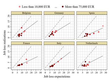
Note: The markers show average quarterly job loss expectations and realisations for ten different income brackets for each country. The brackets are not equally spaced but ordered by increasing intensity of red. The solid lines show weighted linear regression slopes by country and the dashed lines mark the 45-degree line of accurate expectations. Source: CES data.
Since we cannot directly distinguish between voluntary and involuntary job loss, the estimate might partially be driven by planned labour market exits. Although we discussed that the question elicits a rather involuntary transition and we focus on prime-aged respondents who have a high labour market attachment, it is still possible that part of the transitions is due to planned inactivity. In model (4) we therefore only consider transitions into unemployment. While the coefficient is indeed smaller, we find a much higher R2 hinting to a weaker but highly predictive relationship between job loss expectations and job loss.
Our coefficient in model (3) is also slightly lower than the 0.08-0.10 found by Hendren (2017) in a linear model, the 0.12-0.15 found by Stephens (2004) or the 0.11-0.14 found by Dickerson and Green (2012). However, these papers used 12-month ahead job loss expectations and job loss. As we discussed before, job loss expectations 12 months ahead are only slightly above 3-month expectations and highly correlated. Hence, we also try to better align the outcome measure by using as outcome any transition to non-employment in any of the following four quarters (model (5)). In this specification, the estimated coefficient is in line with previous results.
Since individual characteristics seem to be important for the relationship between job loss expectations and realisations, we report the results when controlling for person-fixed effects in an OLS specification in Table A1 in the Appendix. However, this limits the analysis to respondents with at least one labour market transition. Due to the short panel in the CES, we therefore assess only a very small and selective sample of the overall survey. Using the previous controls for this sample in model (1) of Table A1 we find already a more than three times larger coefficient than in model (3) of Table 4 (our baseline specification). However, when controlling for person-fixed effects the coefficient becomes even larger. At the same time, the share of between-group variance to the overall variance (rho) is less than a third for this selective subgroup of job switchers.
Finally, in the same table we assess any non-continuity of the independent variable by aggregating the continuous expectations into eleven bins. This shows that job loss expectations above a level of 60% have a consistently higher probability of job loss than respondents with expectations close to zero. In particular, respondents with close to 100% job loss expectations have a considerably higher probability to not be employed three months later.
Having asserted the consistency and predictability of job loss expectations, we will investigate in the remainder of the paper how job loss expectations, and in particular the errors individuals make in estimating their probability of job losses, affects consumption behaviour.
5 Empirical approach
Since our estimation approach closely follows a standard interpretation of the PIH, we shortly reproduce its main conclusion to illustrate the validity of our empirical approach (following the interpretation by Hall (1978)). We consider a set of agents i (we drop the index for readability) with rational expectations who maximise their lifetime utility subject to a standard budget constraint:
T-t
max Et X ßsu(ct+s) subject to: at+1 = (yt + at - ct)(1 + r) ?t < T and aT+1 = 0 (1)
{ct+s}Ts=0-t s=0
The agents maximize the sum of their utility of consumption u(ct) of all future periods discounted by ß. The per-period budget constraint states that assets in the next period at+1 are equal to the interest-bearing (at fixed rate r) residual of income yt and current assets at less the current period’s consumption. When assuming a quadratic utility function and ß(1+r) = 1, one can show that the Euler equation ct = Et(ct+1) holds for every period t. Using this and solving the budget constraint forward gives the simplest closed-form specification of the PIH:
![]() (2)
(2)
In this standard formulation, the PIH states that consumption is proportional to the level of current assets as well as the expected path of current and discounted future income. First differencing leads to the following expression for consumption changes between t and t + 1:
 (3) Consumption changes ?ct are negatively affected by the current income expectation error and by the change of expectations about discounted future income. Hence, a displacement shock affects the consumption choice via its impact on today’s income as well as the expected future income path. The latter depends on the persistence of the income shock, which is determined by the (expected) employment and unemployment duration.
In order to see this more clearly, we can assume a simple income process conditional on the worker’s employment status. Income yt of employed workers is determined by a per-period wage rate wt, which follows a standard income process of the following form:
![]() with pt = pt-1 + ?t (4)
with pt = pt-1 + ?t (4)
where ![]() and
and ![]() are independent transitory and persistent income shocks.
are independent transitory and persistent income shocks.
An employed worker becomes unemployed with firing probability ft and an unemployed worker becomes employed with hiring probability mt. In case a worker is unemployed, her income is reduced to a share x ? [0,1]. The share x can be interpreted as the replacement rate of unemployment benefits as a share of the worker’s latest income. The income processes can therefore be summarised in the following value functions depending on the employment status, employed (e) or unemployed (u):
 and wt for t = T
(5)
 and xwt for t = T
Since we discuss job loss and job loss expectations, we focus on workers who are employed in period t. Then, workers can either remain employed (with probability (1 - ft+1)) or become unemployed (with probability ft+1). If we call f^t+1 ?{0;1} the realisation of the displacement shock in t + 1 and Et(ft+1) its ex-ante expectation, then one can show that for the average income change across individuals (where the shocks it and ?it average out):
 (6)
(6)
where we assume ?? > t + 1 : f0 = Et+1(f?) = Et(f?) and m0 = Et+1(m?) = Et(m?).9
The individual consumption change therefore depends besides the current period realisations of it and ?it on the difference of the expected job loss probability and its realisation. The higher the ex-ante expectations of this job loss and hence the lower the income expectations, the lower the consumption drop. If a displacement is fully predicted (Et(ft+1) = f^t+1 = 1), there is no change in consumption behaviour. However, if a displacement is not fully expected, i.e.
Et(ft+1) < 1, then consumption is negatively affected (and vice versa for non-displacement). In this specification, the impact on consumption depends on the latest permanent income pt, the unemployment replacement rate x as well as a discount factor.
Assuming for simplicity it and ?it to be zero, using Equations 2 and 3 consumption growth of employed workers can be expressed as:
 (7)
(7)
where . It is decreasing

9This implies that there is no effect of the current realisation of ft+1 on expected future firing or matching probabilities. See also discussion below.
10Today’s consumption (in the denominator) negatively depends on job loss expectations. This implies that workers with higher job loss expectation have a higher consumption growth given the same expectation error. Empirically, however, most workers have low job loss expectations. We discuss any potential non-linearity later in the results section.
in the (perceived) future transition rates (m0 and f0), the level of wealth at (relative to income) and increasing in age (T - t). Accordingly, in Section 7 below we assess the impact of these model predictions by splitting the sample across different dimensions relating to the (perceived) labour market situation, wealth and age.
For the overall assessment of the PIH, we follow the specification of Equation 7 closely to assess the reaction of consumption to the unexpected part of a job loss. To this aim, we construct a variable to capture the "expectation error" (Exp_error) of displacement (Stephens 2004):
Exp_errorit = Et[P(Job_lossit+1)] - 1(Job_lossit+1) ? [-1,1] (8)
The expectation error of individual i at time t is given by the difference of the elicited expected probability and an indicator capturing the actual realisation of job loss in line with Equation 7. The expectation error reaches the value 1 for individuals who unexpectedly remain employed. On the contrary, it reaches -1 for individuals who unexpectedly lose their job. Values of zero indicate a fully matched expectation.
We then estimate a linear model of the following form:
 (9) Here, ?cit+1 = cit+1-cit depicts the consumption change between t+1 and t in logarithmic growth terms. Xit is a matrix of controls. They capture the effect of shifts in consumption preferences that might affect consumption growth for instance over the life cycle or due to differences in household composition. For all sets of results, we include the same set of controls as used in Table 4. This includes a full set of country- and date-fixed effects. In addition, we control for the number of periods a worker took part in the survey in order to capture potential effects of "survey fatigue". Finally, ? denotes a constant and it the residual error term.
The larger the value of the expectation error, the larger should be the reaction of consumption. In case of consumption being totally unresponsive to expectation errors, the beta coefficients should be insignificantly different from zero. In case of a reaction of consumption, this model captures a symmetric effect of an unexpected income shock given that the worker is displaced or not. In terms of Equation 7, ß should be equal to (1 - x)?t.
 In order to assess any non-linearity of positive and negative expectation errors, Stephens (2004) proposed to separate positive and negative error values. In addition, he adds a job loss dummy to his equation to differentiate any average effect of job loss from the actual expectation error. Since negative and positive expectation errors occur only in case of job loss or nonloss, respectively, this specification is equivalent to allowing for an interaction term between expectation errors and job loss in the regression.[9]Hence, using this specification we allow the consumption growth of both displaced and non-displaced workers to have a different level as well as slope:
 (10)
(10)
where Exp_errorit+ = max{Exp_errorit,0} ? 0 is larger than zero for unexpected nondisplacement and Exp_errorit- = min{Exp_errorit,0}? 0 is smaller than zero for unexpected job loss.
Here, ß1 captures the effect of a respondent who expected to lose her job but did not. According to the standard PIH, consumption should increase following a forgone displacement and hence ß1 should be positive. ß2 and ß3 capture the effect of a job loss. In case the job loss is fully anticipated (Exp_errorit- = 0), ß3 captures the average consumption response. In theory, there should be no effect at t + 1 of a displacement that was already fully anticipated in t since consumption should be adjusted at the time of the news. We show that this is the case for our main results and drop the job loss dummy for all additional tables in order to simplify the interpretation of the overall effect of a (partially) unexpected job loss. This consumption response is then captured by ß2. As explained above, the PIH predicts a negative response of consumption to a persistent negative income shock. However, the strength of this effect might differ across individuals depending for instance on their ability to insure this income risk (e.g. via social security or on household level) as well as their re-employment probability. Both factors affect the level and duration of the income shock. We assess this heterogeneity using the vast amount of individual characteristics of the CES in Section 7.
Figure 5: Distribution of expectation errors
Note: The figure on the left shows a histogram of the expectation error. The figure on the right shows a histogram only for workers who lost their job in t +1. Source: CES data.
6 Results
Our estimation approach hinges on the errors respondents make about their job loss expectations in relation to their actual job loss. Individuals that do not lose their jobs can have only positive errors, whereas individuals that lose their jobs can have only negative errors. Most respondents have zero or very small job loss expectations. Since job loss is a rare event, these expectations are mostly in line with realisations. Accordingly, the majority of respondents have zero or only marginally positive expectation errors (see left side of Figure 5)[10]. At the same time, respondents who lose their job are often surprised by this. As the right side of Figure 5 shows, more than 30% of all displaced respondents did not expect to lose their job one quarter before. However, the shares of fully unanticipated displacements and non-displacements are broadly similar.
In addition, the error does not seem to be strongly correlated with socio-economic characteristics or current and past consumption patterns. Table A3 shows the R2 values of OLS regressions of the covariates explained above, including income, tenure, country, and date dummies, on the expectation error. Overall, these covariates explain only around 2% of total variance. This share increases to around 18% for the negative expectation error, if considered separately. The inclusion of current or lagged consumption also seems not to increase the predictability of the error. In addition, Figure A3 shows that the predictive power is not strongly heterogeneous across error levels. Nevertheless, we control for these covariates in our regression Table 5: Consumption in the CES
No job loss | Job loss | ||
Food consumption | 6068.0 | 5169.3 | 6030.6 |
(3386.0) | (3378.7) | (3390.4) | |
Total consumption | 19026.4 | 15501.8 | 18878.8 |
(12022.5) | (10905.0) | (11998.4) | |
Savings | 5237.6 | 4702.1 | 5214.5 |
(8009.2) | (7854.3) | (8003.2) | |
Food consumption growth | 0.00308 | -0.0160 | 0.00236 |
(0.409) | (0.474) | (0.412) | |
Total consumption growth | -0.00363 | -0.0383 | -0.00494 |
(0.418) | (0.494) | (0.421) | |
Savings growth | 0.00426 | -0.0241 | 0.00323 |
(1.161) | (1.520) | (1.176) |
Note: Average annualised consumption and savings of households by displacement status of respondent in t +1 weighted by population weights. All growth variables are defined as logarithmic growth between t and t +1. Quarterly savings have been annualised and log-normally imputed from 11 brackets. Total and food consumption growth are trimmed at their country-specific 2 and 98 percentiles. Standard deviations in brackets. Source: CES data.
framework to capture any potential level or taste differences across groups.
Household spending during the last month is elicited quarterly in the CES broken down into 12 different categories.[11]We first estimate the impact of job loss expectation errors on food consumption. This includes food consumed both at home and outside (in cafes, restaurants, and canteens, including take-out). Food consumption is a frequently used variable in assessing the impact of job loss on consumption due to lack of other consumption data in previous studies (see Hall and Mishkin 1982, Shapiro 1984 or Zeldes 1989 who use food consumption due to the lack of total consumption in the Panel Study of Income Dynamics (PSID)). Focusing on food consumption allows us to compare our estimates to previous results. For the same reason, we annualise total spending in January 2020 EUR and trim it at the 99th percentile. The average annual food consumption is around 6,000 EUR (see Table 5), which is a third less than the converted 9,200 EUR reported by Stephens (2004) for the US. Displaced workers have a lower level of food consumption already prior to their job loss and experience an average drop in consumption of 1.6 log points after their displacement. However, the growth is measured with a large degree of uncertainty, despite us trimming all consumption growth measures at the countryspecific 2 and 98 percentile. This might be due to the caveats related to the measurement of consumption which have also been reported for other survey data sets (see e.g. Shapiro 1984).
The results of our regression on food consumption growth are reported in Table 6. The overall effect of the expectation error following the regression in Equation 9 is shown in column 1. We find a small positive coefficient of the expectation error, which implies that an unexpected job loss reduces the growth of food consumption. When allowing for non-linearity in expectation errors in model 2 as specified in Equation 10, a positive surprise is not related to any adjustment of food consumption. This is despite our data referring to the period of the COVID crisis, when we might have seen higher though unrealised displacement risk in Europe due to the widespread use of job retention schemes. This should allow us to identify the effect of positive expectation errors more precisely.
Stephens (2004) argues that the effect of the positive expectation error should be smaller than the effect of the negative error. Despite a forgone displacement at t + 1, the job might remain at risk in the future which implies higher precautionary savings (see Christelis et al. (2019) for some empirical evidence on this). Hence, consumption might react positively to the information that the job is retained, but only to a lesser extent be affected by the path of future income expectations. This is in line with the observation that for most respondents with a positive expectation error this error is small (see Table 5). Many respondents expect a very small positive probability of job loss that is regularly not realised. This might represent a permanent baseline risk that might already be incorporated in the optimal consumption path and therefore does not induce a consumption response in case of a forgone displacement.
Furthermore, a heterogeneous effect could be driven by a persistent "learning" effect of job loss on the future path of job loss (or finding[12]) expectations. As shown in Equation 7, consumption growth is also affected by expectations about future labour market stability. In case the expected job finding and loss probabilities (m0 and f0) depend on the most recent realisation of ft, there could be "learning about job stability" or "fall off the job ladder" effects. In this case, displaced workers might adjust downward their expectations about their future labour market success. This could imply a differential impact of realised and non-realised job loss expectations and partially explain an asymmetric effect of positive and negative expectation errors.
Descriptively, we see that workers who have been displaced in the past also have higher job loss expectations after re-employment than workers who were never displaced. As can be be seen in Figure 6, job loss expectations are higher for re-employed workers, indicating a higher level Figure 6: Job loss expectations by displacement status
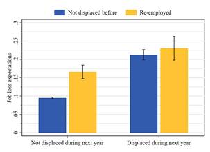
Note: Average job loss expectations by displacement status. Workers who have not reported a displacement before in blue and workers who reported a displacement before and are currently employed in yellow. The left set of bars show workers who did not report a nonemployment during the next four quarters, the right set of bars show workers who did. Confidence bars show 95% standard errors bands. Source: CES data.
of expected displacement risk. This might partially drive the different consumption response of workers with positive and negative expectation errors. Workers who lose their job expect a lower job stability also in the future. This is even the case for workers who are consecutively not displaced (see left bars) and therefore less likely to be adversely selected into displacement and subsequently unstable jobs.[13]
Unlike for positive expectation errors, we find a larger but only marginally significant effect for negative expectation errors.[14]Unexpected displacements are related to a decrease in food consumption by up to 4.4 log points. In model 3 we separate the average effect of a displacement from the expectation error in line with Stephens (2004). We do not find any indication for a large effect of displacement itself, although there is a high degree of estimation uncertainty. While the coefficient of the negative expectation error remains insignificant, the estimate is only slightly smaller than the previous value.[15]These results are therefore in line with the predictions of the Table 6: Job loss expectations and food consumption growth
(1) | (2) | (3) | |
Expectations error | 0.0175 (0.0120) | ||
Positive errors | -0.0040 | -0.0041 | |
(0.0141) | (0.0141) | ||
Negative errors | 0.0445* | 0.0398 | |
(0.0221) | (0.0435) | ||
Displacement | -0.0043 (0.0343) | ||
Country FE | Yes | Yes | Yes |
Date FE | Yes | Yes | Yes |
Controls | Yes | Yes | Yes |
N | 37303 | 37303 | 37303 |
Unique N | 9559 | 9559 | 9559 |
N displaced | 1123 | 1123 | 1123 |
Neg. error | -0.82 | -0.82 | -0.82 |
R2 | 0.01 | 0.01 | 0.01 |
Note: The table depicts the results of an OLS regression. The dependent variable is the logarithmic growth of food consumption in euros between t and t +1. Robust standard errors clustered on individual level in parenthesis. "Neg. error" is the average of the negative values of the expectation error. Stars denote significance levels of two-sided t-tests. * p < 0.1, ** p < 0.05, *** p < 0.01
PIH and point at a role of elicited job loss expectations in the change of consumption paths.
As noted, the results in model 2 are small and only marginally significant. While the previous literature has focused on the reaction of food consumption, this was mostly due to data limitations and has repeatedly been criticised. One caveat in using food consumption to assess the effect of displacement is that the elasticity of food consumption as a necessity good might be lower than that of other consumption items. Therefore, it might be less sensitive to income changes than other, more discretionary consumption items and therefore not representative for the consumption response following a job loss. Similarly, using food consumption to assess the PIH implicitly assumes additive separability of food and other consumption items in the per-period utility function (see Hall and Mishkin 1982). If this is not the case, our estimates of consumption effects are systematically biased. Finally, there is some evidence that food consumption might be more strongly affected by measurement error (Ahmed et al. 2006).
In order to tackle these potential issues, we complement our results with a more comprehensive measure of consumption. The CES elicits in a quarterly frequency consumers’ household expenditure across 12 separate categories during the last month. Our measure of total consumption is based on the aggregation of 11 of these expenditure categories in the CES Figure 7: Average consumption growth by expectation error
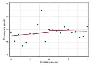
Note: The figure shows the weighted average of logarithmic consumption growth by 21 bins of expectation errors (from -1 to 1 in steps of .1). The regression lines exclude zero and allow for a discontinuity at zero. Source: CES data.
excluding only housing expenditure.[16]The elasticity of these consumption items might be larger than the elasticity of food consumption in case of (unanticipated) displacement (see Table 5).[17]
For displaced workers, consumption and income seem to react to the expectation error in line with the prediction of the PIH (see Figure A2). Consumption of workers with high job loss expectations, and therefore with an error that is closer to zero, seems to drop to the level at displacement already in the quarter before layoff. In line with this, average consumption growth seem to be lower for workers with lower expectation errors (see Figure 7). Similar to the case of food consumption, this seems particularly pronounced for negative expectation errors.
Table 7 shows the results of our regression on the total consumption basket. We still do not find any significant effect of positive expectation errors. However, we find a positive coefficient of the negative expectation error in our baseline specification (column 2). Relative to average total consumption (around 19,000 EUR) the coefficients of model 2 are larger than before and significant at the 5% level. This is in line with the hypothesis that food consumption is less elastic to job loss in the euro area than in the US.[18]
The coefficient also remains positive and significant when controlling for the average Table 7: Job loss expectations and total consumption
(1) | (2) | (3) | (4) | (5) | |
Expectations error | 0.0156 (0.0123) | ||||
Positive errors | -0.0238 | -0.0227 | -0.0339 | ||
(0.0145) | (0.0145) | (0.8962) | |||
Negative errors | 0.0655** | 0.0972* | 0.1259** | ||
(0.0216) | (0.0414) | (0.0417) | |||
Displacement | 0.0289 | -0.0415* | |||
(0.0329) | (0.0175) | ||||
High pos. errors | 0.0087 (0.8936) | ||||
Low neg. errors | -0.0878 (0.0470) | ||||
Country FE | Yes | Yes | Yes | Yes | Yes |
Date FE | Yes | Yes | Yes | Yes | Yes |
Controls | Yes | Yes | Yes | Yes | Yes |
N | 36564 | 36564 | 36564 | 36564 | 36564 |
Unique N | 9463 | 9463 | 9463 | 9463 | 9463 |
N displaced | 1112 | 1112 | 1112 | 1112 | 1112 |
Neg. error | -0.81 | -0.81 | -0.81 | -0.81 | -0.81 |
R2 | 0.01 | 0.01 | 0.01 | 0.01 | 0.01 |
Note: The table depicts the results of an OLS regression. The dependent variable is the logarithmic growth of total consumption in euros between t and t +1. Robust standard errors clustered on individual level in parenthesis. "High pos. errors" ("Low neg. errors") denotes the coefficient of an interaction term of above (below) median non-negative (negative) expectation errors. "Neg. error" is the average of the negative values of the expectation error. Stars denote significance levels of two-sided t-tests. * p < 0.1, ** p < 0.05, *** p < 0.01
displacement effect in a robustness check (model 3). Most importantly, our results for total consumption show that the negative effect of unexpected job loss on consumption (growth) is not driven by the average displacement effect itself. Instead, the negative expectation error is significantly affecting consumption growth. This again is evidence in line with the PIH.[19]In a robustness exercise, we ran more parsimonious specifications with different sets of taste shifters (see Table A2 in the Appendix). The coefficients seem to be consistently estimated even when only controlling for date and country effects as well as when controlling for household composition or lagged consumption.
The semi-elasticity of consumption after a displacement is sizeable. On average, consumption drops by 6.6 log points in case of a fully unexpected displacement. One should recall here the right-hand side panel of Figure 5, which shows that about half of the workers experiencing a job loss have no or very small job loss expectations ex ante and thus are fully surprised by their displacement. Table 2 shows that the average displaced worker has a job loss expectation of around 25%. This is in line with the analysis by Stephens (2004) who reports a 32% average probability in the US in the early 1990s.[20]In our regression sample the average negative expectation error is -0.81. Multiplying this with the estimated coefficient gives an average drop of consumption by 5.3 log points on job loss.[21]
We further probe our results by analysing the behaviour of savings and consumption and whether expectation errors could be correlated with individual characteristics. Savings tend to increase with job loss expectations. Individuals who report an increase of their job loss expectations of at least 10 percentage points more frequently report an increase in their savings.[22]This result supports the view that consumers who expect to lose their jobs save more in order to smooth their consumption pattern, in line with the PIH, dampening the effect of displacement on consumption as shown in our results.
Overall, contrary to earlier studies, we find a significant relationship between negative expectation errors and consumption. There could be a range of reasons for this finding. First, we are able to exploit the large (and still growing) sample size of the CES across a variety of different labour markets. Previous literature analysing the consumption effect of job loss expectations often employed the US PSID (Shapiro 1984, Hall and Mishkin 1982, Zeldes 1989) or HRS data (Stephens 2004, Haider and Stephens 2007, Hendren 2017). Hence, it was focused on one specific labour market and a limited number of observations.[23]The CES instead allows for a cross-border analysis capturing a wide range of institutional settings. Therefore, our estimates are based on a larger set of observations and variation potentially strengthening identification.
Second, the preceding COVID shock increased uncertainty about unemployment risk and duration, since the shock and lockdowns hit different workers and occupations compared to "usual" recessions (see e.g. Mongey et al. (2021)). Although some effects were pointing in a similar direction as during previous recessions, for instance a reduction of expenditure on tourism or restaurants, the magnitude and speed of the closures were unprecedented. At the same time, other sectors that are usually sensitive to business cycle dynamics such as manufacturing were much less affected. This means that expectation errors might be larger than in previous recessions. Some workers who expected to lose their jobs given previous crisis experiences were not so much affected, while others were much more affected. This might have improved the estimate of the "unexpectedness" of job loss but could also increase the noise in our data.[24]At the same time, our focus is on the recovery period after the COVID shock and the strong fiscal reaction in the form of job retention schemes or fiscal support to firms muted the impact of the shock on the labour market. Many workers kept a large part of their income throughout the COVID period. Unfortunately, we cannot compare our results to pre-COVID trends. However, the strong fiscal support and fast economic rebound should have rather weakened the expectation effect of displacement. Hence, finding an effect of negative expectation errors makes us confident that there is a significant impact of unexpected job loss on consumption.
Another difference between US data and our data is the higher unemployment persistence in Europe, and therefore higher persistence of the displacement shock. The persistence of the income shock is an important determinant of the predicted effect of the PIH. Therefore, the on average higher unemployment rates and duration in Europe are important factors in determining the strength of the expected consumption response. We show in the following section that the (perceived) persistence of the income shock is indeed an important driver of the estimates.
7 Decomposing expectation effects
We exploit the scope of the CES by interacting the positive and negative expectation errors with various covariates. As we illustrated in our model above (see Section 5), there are various factors that should affect the strength of the consumption response to an unexpected job loss. Following the results of Equation 7, we assess the effects of (perceived) unemployment persistence, age and wealth in turn. Due to the short time period and limited number of displacements in our data, the precision of our estimates is rather low. Nevertheless, limiting ourselves to two subgroups for each split and finding consistent results across estimations makes us confident that this analysis can support the interpretation of our findings.
First, the perceived prevalence of unemployment affects the re-employment probability of workers. Prior research has shown that individuals’ job finding rates are affected by aggregate labour market conditions.[25]Since we only directly observe job finding expectations for a small subset of workers, we use the perceived unemployment rate in the worker’s country as an indicator for this expected unemployment duration and hence as a proxy for the persistence of the income shock. We cluster workers with perceptions above and below the median perceived unemployment rates in their country (see Table 8) and interact the expectation errors with these groups. As illustrated in the model above, the sensitivity of consumption with respect to the expectation error should be higher for workers who expect lower job finding rates and therefore higher unemployment persistence.
Consistent with this, we find that the effect of negative expectation errors on total consumption is stronger for displaced workers who perceive the unemployment rate to be above their country median (see Table 8). When running a t-test for significant differences between the two coefficients, the difference is significant at the 5% level (see "P value" in the table). This confirms that the re-employment probability is an important driver of the consumption response of workers who were unexpectedly displaced. As the PIH predicts, consumption is very sensitive to persistent changes of the income path. If the expected unemployment duration is long and Table 8: Job loss expectations and consumption - by perceived unemployment rate
Food | ||
Low perceived UE × Positive errors | -0.0090 | -0.0241 |
(0.0195) | (0.0220) | |
High perceived UE × Positive errors | 0.0020 | -0.0220 |
(0.0202) | (0.0192) | |
Low perceived UE × Negative errors | 0.0411 | 0.0186 |
(0.0299) | (0.0293) | |
High perceived UE × Negative errors | 0.0485 | 0.1191*** |
(0.0319) | (0.0314) | |
Country FE | Yes | Yes |
Date FE | Yes | Yes |
Controls | Yes | Yes |
N | 37303 | 36564 |
Unique N | 9559 | 9463 |
N displaced | 1123 | 1112 |
Neg. error | -0.82 | -0.81 |
P value | 0.86 | 0.02 |
R2 | 0.01 | 0.01 |
Note: The table depicts the results of an OLS regression. The dependent variable is the logarithmic growth of food consumption (column 1) and of total consumption (column 2) in euros between t and t +1. "Low (high) perceived UE" are workers with below (above) median unemployment rate perceptions in their country. Robust standard errors clustered on individual level in parenthesis. "Neg. error" is the average of the negative values of the expectation error. Stars denote significance levels of two-sided t-tests. * p < 0.1, ** p < 0.05, *** p < 0.01
the perceived job finding probability is low, income is expected to be subdued for a longer period and consumption reacts stronger to errors in ex-ante job loss expectations.
After showing that expected unemployment persistence matters for the predictions of the PIH to hold, we next look at age. Unlike Stephens (2004) and others using HRS data, which only covers workers above age 50, we can also assess the effect of unexpected displacement on the consumption of younger workers. Therefore, we split the sample around its median age of 45. Indeed, we find that workers above the age of 45 have a stronger response of consumption to unexpected job loss (Table 9). While the coefficients are closer for total consumption, the difference is much larger for food consumption.
This heterogeneity could work through different channels. First, older workers have been shown to have a higher unemployment duration (e.g. Neumark et al. 2019). These results then are again in line with the notion that more persistent income changes affect consumption behaviour to a larger extent. However, there could be also other factors that affect the consumption response of older workers in this or the opposite direction, such as taste shifts, the optimisation time frame or precautionary savings. First, the direction of the impact of taste shifts is ambiguous Table 9: Job loss expectations and consumption - by age group
Food | ||
Low age × Positive errors | 0.0101 | -0.0164 |
(0.0205) | (0.0207) | |
High age × Positive errors | -0.0196 | -0.0327 |
(0.0170) | (0.0179) | |
Low age × Negative errors | -0.0071 | 0.0543 |
(0.0306) | (0.0309) | |
High age × Negative errors | 0.1144*** | 0.0800** |
(0.0301) | (0.0287) | |
Country FE | Yes | Yes |
Date FE | Yes | Yes |
Controls | Yes | Yes |
N | 37303 | 36564 |
Unique N | 9559 | 9463 |
N displaced | 1123 | 1112 |
Neg. error | -0.82 | -0.81 |
P value | 0.00 | 0.54 |
R2 | 0.01 | 0.01 |
Note: The table depicts the results of an OLS regression. The dependent variable is the logarithmic growth of food consumption (column 1) and of total consumption (column 2) in euros between t and t+1. Workers aged 25 to 44 are classified as "low age" and workers aged 45 to 59 as "high age". Robust standard errors clustered on individual level in parenthesis. "Neg. error" is the average of the negative values of the expectation error. Stars denote significance levels of two-sided t-tests. * p < 0.1, ** p < 0.05, *** p < 0.01
and hard to assess. However, some of our control variables should capture the part of these shifts for instance related to household composition or income. Second, a job loss has a stronger effect on future income of older workers due to their shorter (working) life (see Equation 7). Since they optimise their consumption path over a shorter horizon (T -t), their consumption response should react stronger to unexpected changes in their income path. Finally, self-insurance against income risk via precautionary savings should have the opposite effect (see e.g. Kaplan and Violante 2010). Older workers should have accumulated a larger share of savings necessary to smooth consumption risk if their utility function exhibits prudence. In this case, Blundell et al. (2008) have shown that the consumption response is muted by a factor that is proportional to the share of labour relative to total wealth. Hence, our results support the notion that the re-employment probability (persistence) as well as the shorter time frame are dominating the counteracting effect of potential precautionary savings.
A final important factor for the effect of unexpected job loss on consumption is the available level of financial means to cushion the impact of the income shock. The more a household depends on current labour income to cover current consumption, the less it is able to react to a negative income shock by running down wealth or precautionary savings. Hence, households with a low level of liquid financial means should react stronger to a persistent income shock (but not permanent, see Kaplan and Violante (2010) or Kaplan et al. (2014)).
We test this prediction by splitting the sample into households with net financial wealth above and below half their monthly income. Households below this threshold have been named "hand-to-mouth", since their liquid financial means cover less than the average balances of just one income period. Financial net wealth is elicited only once in the CES (in November 2021) and household income only once upon joining the panel. Hence, we have to assume a constant wealth level over the survey horizon.[26]We add up the midpoints of 8 bracketed wealth categories covering current and saving accounts, cash, stocks, mutual funds, bonds, and other financial assets, and deduct any outstanding liabilities such as credit lines, overdrafts, or loans (no mortgages).
Following these definitions, we find that median net wealth is only slightly above 5,000 EUR. This is approximately equivalent to 4 months of household consumption of an average displaced worker. However, due to the availability of unemployment benefits in many European countries, the income shock is usually not equivalent to 100% of permanent income. In relation to the monthly income of households, we find that the distribution for January 2022 (first quarterly survey after the wealth survey in November 2021) looks similar to the one reported by Kaplan et al. (2014) for the largest four euro area countries (see Figure 8). Our measure contains somewhat more households with negative wealth levels, but at the same time there are fewer households with around zero net wealth. Following the definition of liquidity-constrained households mentioned above, we find that 33% of households can be classified as "hand-tomouth". This is in line with findings by Kaplan et al. (2014) for the US but slightly above the share of 20-30% they found for the largest euro area countries using data from the Household Finance and Consumption Survey (HFCS).
When interacting the expectation errors with a HtM dummy, we find evidence of a consumption smoothing effect depending on available financial means (Table 10). In line with the PIH, the negative consumption response is stronger for households with low liquid wealth levels. While high wealth individuals experience no significant sensitivity of consumption to negative expectation errors, we find a significant effect for "hand-to-mouth" workers’ total consumption.
Figure 8: Distribution of liquid wealth relative to monthly income
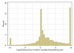
Note: Histogram of net liquid financial wealth in November 2021 relative to monthly household income at the time of the first survey of the household. The distribution is winsorised at -10 and 10. Source: CES data.
Table 10: Job loss expectations and consumption - by wealth level
Food | ||
HtM × Positive errors | -0.0032 | -0.0295 |
(0.0192) | (0.0197) | |
No HtM × Positive errors | -0.0051 | -0.0184 |
(0.0193) | (0.0198) | |
HtM × Negative errors | 0.0471 | 0.0852** |
(0.0305) | (0.0305) | |
No HtM × Negative errors | 0.0421 | 0.0477 |
(0.0316) | (0.0303) | |
Country FE | Yes | Yes |
Date FE | Yes | Yes |
Controls | Yes | Yes |
N | 37303 | 36564 |
Unique N | 9559 | 9463 |
N displaced | 1123 | 1112 |
Neg. error | -0.82 | -0.81 |
P value | 0.91 | 0.38 |
R2 | 0.01 | 0.01 |
Note: The table depicts the results of an OLS regression. The dependent variable is the logarithmic growth of food consumption (column 1) and of total consumption (column 2) in euros between t and t+1. Households with net liquid financial wealth levels below half their monthly income are classified as "hand-to-mouth" (HtM), while households above this limit are not (no HtM). Robust standard errors clustered on individual level in parenthesis. "Neg. error" is the average of the negative values of the expectation error. Stars denote significance levels of two-sided t-tests. * p < 0.1, ** p < 0.05, *** p < 0.01
8 Conclusion
The monitoring of expectations and confidence indicators has been expanding quickly in the last years. We use the novel CES data to investigate the role of job loss expectations on consumption. Those expectations behave in a manner that is consistent with income expectations and the actual realisations of job loss. In our analysis we show that expectations have consistent and significant predictive power for future labour market and consumption patterns. At the same time, we show that actual job loss is for many workers an event that is difficult to predict. For those workers their reaction is aligned with the PIH. Individuals that did not fully anticipate their job loss adjust their consumption at dismissal significantly more than consumers who did anticipate a job loss. At the same time, we do not find that positive errors lead to an increase in consumption. As discussed, this asymmetry could be related to the continuing risk of job loss or updating of job loss expectations. Overall, this implies that job loss risk has important and asymmetric consequences for consumption and savings behaviour.
The persistence of unemployment seems to be an important driver of our results. We show that for workers with higher unemployment rate perceptions and older workers the effect of negative expectation errors on the fall in consumption tends to be larger. This is in line with the interpretation that the consumption response is proportional to the persistence of the income shock and therefore the probability of re-employment - consistent with the theoretical predictions of the PIH.
Our results thus add to the growing literature on the effect of expectations on individuals’ decisions, with a possible impact on macroeconomic dynamics. Job loss expectations help to predict actual job loss and consumption behaviour even before the labour market effects materialise. At the same time, the asymmetry we show in our paper implies that while policies aimed at preventing job loss (such as job retention schemes) support consumption, they are not sufficient to fully prevent a fall in consumption of workers who unexpectedly keep their jobs. As the risk of unemployment remains, consumers do not significantly increase their consumption path following a forgone job loss.
Thus, in an environment of elevated uncertainty with increased job loss expectations, consumption is likely to remain lower even if employment is protected. This might explain developments in consumption during the COVID pandemic. While job protection schemes prevented a larger fall in consumption than that it would have occurred in the presence of a bigger fall in employment, consumption only returned to pre-crisis levels three years after the start of the pandemic. This is despite the early recovery in employment and the fall in unemployment to record low levels.
References
Ahmed, N., Brzozowski, M., and Crossley, T. F. (2006). Measurement errors in recall food consumption data. Technical report, IFS Working Papers.
Balleer, A., Duernecker, G., Forstner, S., and Goensch, J. (2021). Perceived and actual labor market risk. mimeo.
Benito, A. (2006). Does job insecurity affect household consumption? Oxford Economic Papers, 58(1):157181.
Blundell, R., Pistaferri, L., and Preston, I. (2008). Consumption inequality and partial insurance.
American Economic Review, 98(5):18871921.
Browning, M. and Crossley, T. (2001). The life-cycle model of consumption and saving. Journal of Economic perspectives, 15(1):322.
Campbell, D., Carruth, A., Dickerson, A., and Green, F. (2007). Job insecurity and wages. The
Economic Journal, 117(518):544566.
Campos, R. and Reggio, I. (2015). Consumption in the shadow of unemployment. European
Economic Review, 78(C):3954.
Carroll, C. D. and Dunn, W. E. (1997). Unemployment expectations, jumping (s, s) triggers, and household balance sheets. NBER macroeconomics annual, 12:165217.
Christelis, D., Georgarakos, D., and Jappelli, T. (2015). Wealth shocks, unemployment shocks and consumption in the wake of the great recession. Journal of Monetary Economics, 72:2141. Christelis, D., Georgarakos, D., Jappelli, T., Pistaferri, L., and Van Rooij, M. (2019).
Asymmetric consumption effects of transitory income shocks. The Economic Journal, 129(622):23222341.
Christelis, D., Georgarakos, D., Jappelli, T., and van Rooij, M. (2020). Consumption uncertainty and precautionary saving. Review of Economics and Statistics, 102(1):148161.
Dias da Silva, A., Dossche, M., Dreher, F., Foroni, C., and Koester, G. (2020). Short-time work schemes and their effects on wages and disposable income. Economic Bulletin Boxes, 4.
Dickerson, A. and Green, F. (2012). Fears and realisations of employment insecurity. Labour
Economics, 19(2):198210.
Dominitz, J. (2001). Estimation of income expectations models using expectations and realization data. Journal of Econometrics, 102(2):165195.
Dominitz, J. and Manski, C. F. (1997). Using expectations data to study subjective income expectations. Journal of the American statistical Association, 92(439):855867.
ECB (2021). ECB consumer expectations survey: An overview and first evaluation. Occasional Paper Series 287, European Central Bank.
Enders, Z., Hünnekes, F., and Müller, G. (2022). Firm expectations and economic activity.
Journal of the European Economic Association, 20(6):23962439.
Georgarakos, D. and Kenny, G. (2022). Household spending and fiscal support during the covid-
19 pandemic: Insights from a new consumer survey. Journal of monetary economics, 129:S1 S14.
Gruber, J. (1997). The consumption smoothing benefits of unemployment insurance. American
Economic Review, 87(1):192205.
Haider, S. J. and Stephens, M. (2007). Is there a retirement-consumption puzzle? evidence using subjective retirement expectations. The Review of Economics and Statistics, 89(2):247264.
Hall, R. E. (1978). Stochastic implications of the life cycle-permanent income hypothesis: theory and evidence. Journal of political economy, 86(6):971987.
Hall, R. E. and Mishkin, F. S. (1982). The sensitivity of consumption to transitory income:
Estimates from panel data on households. Econometrica, 50(2):461481.
Hendren, N. (2017). Knowledge of future job loss and implications for unemployment insurance.
The American Economic Review, 107(7):17781823.
Jacobson, L. S., LaLonde, R. J., and Sullivan, D. G. (1993). Earnings losses of displaced workers.
The American economic review, pages 685709.
Jappelli, T. and Pistaferri, L. (2000). Using subjective income expectations to test for excess sensitivity of consumption to predicted income growth. European Economic Review, 44(2):337 358.
Kaplan, G. and Violante, G. L. (2010). How much consumption insurance beyond self-insurance?
American Economic Journal: Macroeconomics, 2(4):5387.
Kaplan, G., Violante, G. L., and Weidner, J. (2014). The wealthy hand-to-mouth. Technical report, National Bureau of Economic Research.
Kroft, K., Lange, F., and Notowidigdo, M. J. (2013). Duration dependence and labor market conditions: Evidence from a field experiment. The Quarterly Journal of Economics, 128(3):11231167.
Manski, C. F. (2004). Measuring expectations. Econometrica, 72(5):13291376.
Manski, C. F. and Straub, J. D. (2000). Worker perceptions of job insecurity in the mid-
1990s: Evidence from the survey of economic expectations. The Journal of Human Resources, 35(3):447479.
McGuinness, S., Wooden, M., and Hahn, M. (2014). The perceived probability of job loss and future labour market outcomes. Industrial Relations Journal, 45(4):329347.
Meghir, C. and Pistaferri, L. (2011). Earnings, consumption and life cycle choices. In Handbook of labor economics, volume 4, pages 773854. Elsevier.
Mongey, S., Pilossoph, L., and Weinberg, A. (2021). Which workers bear the burden of social distancing? The Journal of Economic Inequality, 19(3):509526.
Mueller, A. and Spinnewijn, J. (2021). Expectations data, labor market and job search. Handbook
Chapter (Draft).
Neumark, D., Burn, I., and Button, P. (2019). Is it harder for older workers to find jobs? new and improved evidence from a field experiment. Journal of Political Economy, 127(2):922970. Penrose, G. and La Cava, G. (2021). Job loss, subjective expectations and household spending.
Technical report, Reserve Bank of Australia.
Pettinicchi, Y. and Vellekoop, N. (2019). Job loss expectations, durable consumption and household finances: Evidence from linked survey data. SAFE Working Paper Series 249, Leibniz Institute for Financial Research SAFE.
Pistaferri, L. (2001). Superior information, income shocks, and the permanent income hypothesis.
Review of Economics and Statistics, 83(3):465476.
Shapiro, M. D. (1984). The permanent income hypothesis and the real interest rate: some evidence from panel data. Economics Letters, 14(1):93100.
Stephens, M. (2001). The long-run consumption effects of earnings shocks. Review of Economics and Statistics, 83(1):2836.
Stephens, M. (2004). Job loss expectations, realizations, and household consumption behavior.
The Review of Economics and Statistics, 86(1):253269.
Zeldes, S. P. (1989). Consumption and liquidity constraints: an empirical investigation. Journal of political economy, 97(2):305346.
9 Appendix
Figure A1: Job loss expectations and realisations by country and income percentile
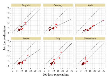
Note: The markers show average quarterly job loss expectations and realisations for ten income percentiles for each country. The percentiles are based on net income (i.e. after tax and compulsory deductions) from all sources, calculated by country and quarter, and ordered by increasing intensity of red. The solid lines show weighted linear regression slopes by country and the dashed lines mark the 45-degree line of accurate expectations. Source: CES data.
Table A1: Robustness: Job loss expectations and job loss realisations
(1) | (2) | (3) | |
E to Non-E | E to Non-E | E to Non-E | |
Job loss expectations | 0.2196*** | 0.3523*** | |
(0.0307) | (0.0478) | ||
Loss_probability=10 | 0.0060 (0.0031) | ||
Loss_probability=20 | 0.0185*** (0.0053) | ||
Loss_probability=30 | 0.0172* (0.0068) | ||
Loss_probability=40 | 0.0155 (0.0098) | ||
Loss_probability=50 | 0.0106* (0.0046) | ||
Loss_probability=60 | 0.0303 (0.0161) | ||
Loss_probability=70 | 0.0623* (0.0249) | ||
Loss_probability=80 | 0.0619** (0.0191) | ||
Loss_probability=90 | 0.1185*** (0.0314) | ||
Loss_probability=100 | 0.1715*** (0.0201) | ||
Country FE | Yes | No | Yes |
Date FE | Yes | Yes | Yes |
Tenure bracket FE | Yes | Yes | Yes |
Income bracket FE | Yes | Yes | Yes |
Other controls | Yes | No | Yes |
Person FE | No | Yes | No |
N | 4373 | 4373 | 40813 |
Unique N | 1172 | 1172 | 9993 |
R2 | 0.03 | 0.05 | |
Rho | 0.30 | ||
Pseudo R2 | 0.10 |
Note: The table depicts in columns 1 and 2 results of an OLS regression. Column 2 includes person-fixed effects and column 1 uses the main regression specification using the same sample. Column 3 shows average marginal effects of a Probit estimation. The dependent variable is job loss in the following quarter. Job loss expectations are defined between 0 and 1 in model (1) and (2), and are put into the closest percentile bin in model (3) (omitted category: Loss_probability =0). Robust standard errors clustered on individual level in parenthesis. "Rho" denotes the between-variance as a share of the total variance. Stars denote significance levels of two-sided t-tests. * p < 0.1, ** p < 0.05, *** p < 0.01

Table A3: Predictability of expectation errors
(1) | (2) | (3) | (4) | (5) | |
Overall | Pos. error | Pos. error incl. consumption | Neg. error | Neg. error incl. consumption | |
N | 40813 | 20712 | 16750 | 1308 | 940 |
Unique N | 9993 | 6538 | 5346 | 1160 | 849 |
R2 | 0.02 | 0.10 | 0.11 | 0.18 | 0.19 |
Note: Adjusted R2 values for regressions on expectation errors - either overall (model 1) or separately for positive (model 2 and 3) and negative (model 4 and 5) expectation errors. Controls include tenure bracket, income bracket, education, gender, age group, partner in household, household size, quarter and country. Models (3) and (5) in addition include current and lagged logarithmic values of total and food consumption. Source: CES data.
Figure A2: Average income and consumption around displacement
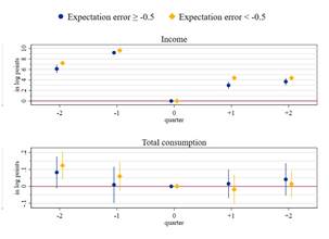
Note: The figure shows the quarterly average personal net income and household consumption (excl. housing) relative to their displacement quarter (t = 0) in logarithmic terms. Estimates are weighted by population weights and the bars depict standard errors at a 95% confidence level clustered on individual level. Source: CES data.
Figure A3: Predicted values of positive and negative expectation error
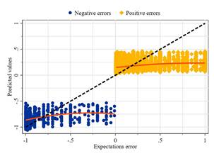
Note: The figure shows the predicted values of the expectation error based on models (3) and (5) in Table A3 relative to its actual value. The red line shows quadratic regression lines separately for the negative and positive predictive values. The black dashed line is the 45-degree line (perfect prediction). Source: CES data.
Details about the household consumption variable in the CES
The CES elicits with quarterly frequency data on household consumption, grouped in twelve categories. The survey question asks about consumption during the last month before the survey is taken. Respondents are provided with an interface where they fill in the sum of their spending (in an open-ended manner) for each category (and are given the opportunity to tick a box if they did not spend any money on the respective category). At the end, respondents are presented with a summary screen, which gives the possibility to review all entries and introduce corrections if some of them are erroneous or imprecise. As the reference period for consumption is one month, the data are annualized. Consumption growth is calculated as quarter-on-quarter growth.
The specific wording of the consumption question is as follows: During <last month>, how much did your household spend on the goods and services listed below? (where "last month" is replaced with the name of the month)
•Food, beverages, groceries, tobacco
•Restaurants (including take-out food, delivery), cafes/ canteens
•Housing (including rent, maintenance/repair costs, home owner/renter insurance, but excluding mortgage payments)
•Utilities (including water, sewerage, electricity, gas, heating oil, phone, cable, internet)
•Furnishings (furniture, carpets), household equipment (textiles, appliances, garden tools), small appliances and routine maintenance of the house (cleaning, gardening)
•Debt repayments (instalments in mortgage, consumer loans, car loans, credit cards, student loans, other loans)
•Clothing, footwear
•Health (health insurance, medical products and appliances, dental and paramedical services, hospital services, prescription and non-prescription medication, personal care products and services)
•Transport (fuel, car maintenance, public transportation fares)
•Travel, recreation, entertainment and culture (holidays, theatre/ movie tickets, club/ gym membership, newspapers, books, hobbies equipment)
•Childcare and education (including tuition fees for child and adult education, costs of after school activities, care of children/ babysitting, but excluding instalments on student loans) • Other expenditures not mentioned above
With this setup, in terms of timing, the job loss expectations and the consumption data can be seen as elicited in nearly the same time period, as the respondents receive the questionnaire only a few days after the end of the reference month for consumption data, and the bulk of responses are received in the first days of the survey.
The food consumption data in the Consumer Expectations Survey are broadly comparable to the same data in the EU SILC survey at country level, in spite of some differences in both surveys’ methodologies. In addition, in ECB (2021), the structure of spending in the CES survey is also found to be in line with the Household budget survey in 2015, although some differences due to the pandemics are observed.
Acknowledgements
We are grateful for many comments and remarks by Francesco D’Amuri, Dimitris Georgarakos and an anonymous referee, all members of the CES core team as well as seminar participants of ECB’s Research task-force on Heterogeneity in macroeconomics, ECB’s CES research seminar and the 6th Annual Workshop of the ESCB Research Cluster 2.
The opinions in this paper are those of the authors and do not necessarily reflect the views of the European Central Bank (ECB) or the Eurosystem.
António Dias da Silva
European Central Bank, Frankfurt am Main, Germany; email: antonio.dias_da_silva@ecb.europa.eu
Desislava Rusinova
European Central Bank, Frankfurt am Main, Germany; email: desislava.rusinova@ecb.europa.eu
Marco Weißler
European Central Bank, Frankfurt am Main, Germany; email: marco.weissler@ecb.europa.eu
Postal address 60640 Frankfurt am Main, Germany
Telephone +49 69 1344 0
Website www.ecb.europa.eu
All rights reserved. Any reproduction, publication and reprint in the form of a different publication, whether printed or produced electronically, in whole or in part, is permitted only with the explicit written authorisation of the ECB or the authors.
This paper can be downloaded without charge from www.ecb.europa.eu, from the Social Science Research Network electronic libraryor from RePEc: Research Papers in Economics. Information on all of the papers published in the ECB Working Paper Series can be found on the ECB’s website.
PDF ISBN 978-92-899-6080-9 ISSN 1725-2806 doi:10.2866/06611 QB-AR-23-054-EN-N
[1] One exception is Balleer et al. (2021) who find households to be somewhat overoptimistic in the sense that they underestimate the job loss probability.
[2] The main analysis uses data after October 2020, which means that the largest variations in the labour market series in consequence of the pandemic occurred before the period we analyse in this paper.
[3] The quarterly survey is fielded in January, April, July and October.
[4] We define employment as full- or part-time employment including temporarily layoffs. Unemployed are respondents without a job but actively looking for a job. Everyone else is considered inactive including workers on extended leave, retirees, students, or caretakers.
[5] The monthly question elicits in five qualitative brackets for expectation of net total household income during the next 12 months.
[6] The monthly question asks in an open-ended manner for income growth expectations in percentage points up to one decimal and limited by the preceding bracketed answer.
[7] Respondents are asked quarterly for their annual work-related income (excluding unemployment benefits) on individual level. The income is elicited in 10 (not equally spaced) brackets from "below EUR 10,000" up to "EUR 75,000 and more". Alternatively, we show in Figure A1 in the Appendix the chart for ten country-specific percentiles based on household net income from all sources that is elicited only once when households enter the survey.
[8] The labour market developments in these countries during the pandemic are relatively similar and thus the pandemic is not likely to have a strong effect on these correlations. All six countries enter the pandemic with relatively low unemployment rates and all but one had a lower unemployment rate at the end of the period of our analysis then before the pandemic. Job retention schemes played a key role in supporting employment and income in all six countries.
[9] To see this, an interaction term in a model without controls could be specified as ?cit+1 = ?+ß~1Exp_errorit+
. In case of no job loss, the marginal effects of the
expectation error on consumption growth are ß1 and ß~1 in both models, respectively. In case of job loss, the marginal effects are ß2 and ß~1 + ß~2. Since ß~1 is identified by the case of non-loss, this leads to equivalent estimates.
[10] Another observation is the strong non-normality and non-linearity of the distribution around zero. We partially cater for this by estimating the regression separately for positive and negative expectation errors and by adding an interaction term for high positive and low negative errors in a robustness check.
[11] For details regarding the nature of spending data in the CES and the survey question formulation, please refer to the Appendix.
[12] Job finding expectations are only elicited for unemployed workers in the CES. Due to the small sample size, we cannot assess their development after changes of employment status.
[13] This difference is also similar in size and significant at the 1% level when controlling for education, gender, age group, partnership status, household size, income, country and quarter.
[14] The values of the negative error are below zero. Hence, a positive coefficient implies a negative effect on consumption.
[15] Stephens finds that after a fully unexpected job loss, food consumption falls by up to 1,260 USD relative to an average of 6,700 USD if positive and negative expectation errors are separated. However, most of this is driven by the average effect of displacement itself instead of the negative expectation error. This is not in line with the PIH that predicts no effect of anticipated job loss but a negative effect of unanticipated job loss.
[16] We restrict our sample of consumption data to workers who also report non-zero food consumption.
[17] While the elasticity of specific larger items like furniture, appliances or holidays might be even larger, considering only these items is not a feasible alternative because these are rare purchases: the large number of zeros in the series would be an issue for constructing consumption growth.
[18] In order to assess any non-linearity in the estimated results, we also interact the errors with a dummy for values above (below) the median non-negative (negative) expectation error (model 5). However, the estimates do not allow for strong conclusions since they are insignificant and strongly dependent on the specified cutoff levels.
[19] For the rest of the paper we do not report the results of the displacement dummy separately in order to simplify the interpretation. In all specifications we ran, the coefficients of the displacement dummy were insignificant.
[20] The unemployment rate in the US stood around 6-8% in the early 1990s. This is also broadly in line with the 7-8.5% in the euro area in 2020 and 2021. However, the measurement and implications of the unemployment status strongly differ between the two areas and hence are not directly comparable.
[21] This is lower than the findings in the HRS for the US. Christelis et al. (2015) find a 10% drop of consumption after a job loss of at least one of the partners in a household during the Great Recession in 2009.
[22] Savings in the CES are only available in brackets. Hence, we define a savings increase as a move from a lower into a higher bracket.
[23] In his consumption analysis using HRS data Stephens (2004) has only 3,509 observations (271 displacements) on 2,432 individuals after applying his sample selection.
[24] The intensive usage of job retention schemes in Europe might cover the fact that - despite a low number of displacements - hours and income dropped and displacement risk increased (Dias da Silva et al. 2020).
[25]Kroft et al. (2013) for instance show that call-back rates are lower in US metropolitan areas with higher unemployment rates. Our sample size is too small to allow for a breakdown of the main regressions in order to identify potential structural cross-country differences. Hence, we focus in the paper on the euro area as a whole (as represented by the six countries in the CES). More recent CES waves (from mid-2022) also cover additional countries and might allow for such an analysis in the future.
[26] This means that financial wealth is measured partially at a different time from the household income and also partially after the displacement. This is therefore a strong caveat of our results. However, the singular elicitation of the wealth and household income variables does not allow for a better time alignment with displacement.

