The consumption impulse from pandemic savings ‒ does the composition matter?
Prepared by Niccolo Battistini, Virginia Di Nino and Johannes Gareis
Published as part of the ECB Economic Bulletin, Issue 4/2023.
Following the outbreak of the pandemic, households in the euro area and the United States accumulated a large stock of savings, in excess of the pre-pandemic trend.[1] Between the first quarter of 2020 and the fourth quarter of 2022, the accumulated stock of excess savings rose steadily to reach 11.3% of trend (gross) disposable income in the euro area. In the United States, the accumulated stock of excess savings reached 13.2% in the third quarter of 2021, before declining to 7.9% in the fourth quarter of 2022.[2] Taken at face value, the large stock of excess savings in both economies suggests the possibility of a substantial consumption impulse, defined as the immediate stimulus to consumption from the potential use of these savings. Moreover, it points to a larger remaining consumption impulse in the euro area relative to the United States, where consumption has expanded by considerably more in the post-pandemic period. Besides the size of the stock, the composition of excess savings plays a key role in determining the implied consumption impulse. This box estimates the composition of excess savings and then calibrates a general equilibrium model with heterogenous agents based on the methodology used by Auclert et al. to gauge the consumption impulse in the two jurisdictions.[3]
Beyond the stock of pandemic savings, the composition of these excess savings matters for two reasons. First, excess savings are allocated across assets with different degrees of liquidity, which is a first (partial equilibrium) determinant of their consumption impulse. Second, the impact of excess savings on the consumption impulse also depends on broader (general equilibrium) dynamics: on the one hand, the dynamic re-distribution of the savings spent by some households to other households prolongs the duration of the consumption impulse; on the other hand, the anticipation by households of this future re-distribution dampens the size of the consumption impulse, as households smooth their consumption patterns over time. Empirical evidence suggests that these partial and general equilibrium effects may play out differently in the euro area and the United States.
Between 2020 and 2022, in the euro area, excess savings were accumulated mostly in illiquid assets, while in the United States these were largely accumulated in liquid assets.In the euro area, between the first quarter of 2020 and the fourth quarter of 2022, excess savings were invested in non-financial assets, such as housing, and in relatively illiquid financial assets, such as stocks and bonds, and were also used to pay back loans. Taken together, these forms of cumulated excess savings rose steadily to reach 10.8% of trend disposable income in the fourth quarter of 2022 (Chart A). By contrast, cumulated excess savings in the (most) liquid financial assets, such as currency and deposits, peaked at 3.7% of trend disposable income in the first quarter of 2021 and then declined significantly to 0.6% in the fourth quarter of 2022. In the United States, the composition of cumulated excess savings at the end of 2022 was remarkably different. Liquid financial assets amounted to 18.5% of trend disposable income, while illiquid assets fell below their pre-pandemic trend by 10.6%, also reflecting a sizeable accumulation of new loans.[4]
Chart A
Allocation of cumulated excess savings across assets
(deviations from the pre-pandemic trend, percentages of trend disposable income)
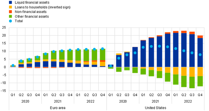
Sources: Eurostat, ECB, Federal Reserve Board and ECB calculations.
Notes: Each entry represents the cumulated value exceeding its trend estimated between 2015 and 2019. Liquid financial assets refer to currency and deposits. Non-financial assets refer to gross capital formation. Other financial assets are calculated as a residual and mainly refer to stocks and bonds.
Over the past three years the stock of excess savings was increasingly concentrated among wealthy households on both sides of the Atlantic. The analysis of the distribution of excess savings across households combines their estimated allocation across assets, discussed above, with survey information on the composition of household portfolios along the net wealth distribution.[5] The implied distribution of excess savings shows an ever greater concentration among relatively high-wealth households, in particular in the United States (Chart B). The share of cumulated excess savings held by households in the top 10% of the distribution rose from less than half in the first quarter of 2020 in both economies to almost two-thirds in the euro area and more than three-quarters in the United States in the fourth quarter of 2022. However, the relatively larger share of excess savings among low-wealth households in the euro area does not imply a higher consumption impulse compared with the United States. This is because the excess savings in the euro area mostly consisted of relatively illiquid assets, including housing wealth and loan repayments, which represent an important share of portfolios for households at the lower end of the distribution.
Chart B
Distribution of cumulated excess savings across household groups
(deviations from the pre-pandemic trend, percentages of trend disposable income)
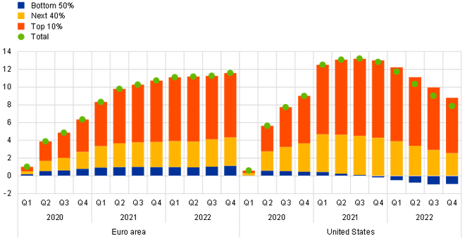
Sources: Eurostat, ECB (including the experimental Distributional Wealth Accounts), US Bureau of Economic Analysis, Federal Reserve Board (including the Distributional Financial Accounts) and ECB calculations.
Notes: The model features three groups of households, corresponding to the bottom 50%, the next 40% and the top 10% of the excess savings distribution. The distribution of excess savings across households is obtained by multiplying the share of assets in the portfolio of each household group (distributional accounts) by the estimated excess savings in each asset class.
A heterogeneous agent model is used to link the estimated distribution of excess savings across assets and households to their consumption impulse, accounting for partial and general equilibrium effects. The model features three groups of households, corresponding to the bottom 50%, the next 40% and the top 10% of the excess savings distribution. Under partial equilibrium, each group decides what share of excess savings to consume or save in each period based on its marginal propensity to consume (MPC), which is assumed to depend on the asset composition of its excess savings. Under general equilibrium, consumption decisions reflect two further mechanisms. First, the savings spent by some households become the income that is financing consumption for other households. As a result, the impulse on consumption is prolonged and it dissipates only slowly, as excess savings “trickle up” towards high-wealth, high-income households, which have a lower MPC. Second, households anticipate the future expansion in aggregate demand and smooth their consumption on impact, with the implied moderating effect being proportional to the MPCs for each household group.[6] This incentivises the accumulation of savings and limits the re-distribution of income, thus expediting the trickling up of excess savings and muting the consumption impulse.[7] In both scenarios, the central bank does not react to the expansion in demand, thus keeping the interest rate fixed. Overall, the potential, model-implied impulse to consumption from the use of excess savings depends on the calibration of two sets of parameters: (i) the MPC for each asset class; and (ii) the share of total income for each group of households (Chart C). The MPC is set to 50% for liquid financial assets and 5% for illiquid assets.[8] The share of income is calibrated at 9%, 55% and 36% in the euro area and 15%, 36% and 49% in the United States for the bottom 50%, next 40% and top 10% of the excess savings distribution respectively.
Chart C
Marginal propensity to consume across assets and income across household groups
(percentages)
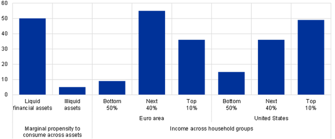
Sources: 2017 Household Finance and Consumption Survey, 2019 Survey of Consumer Finances, Slacalek et al., op. cit., and ECB calculations.
Note: Liquid financial assets refer to deposits and currency, illiquid assets include non-financial and other financial assets, as well as loans to households (inverted sign).
The consumption impulse from pandemic savings has declined in both economies and has been lower in the euro area compared with the United States. Under partial equilibrium, the model assumes that household decisions do not account for the re-distribution of income and the response in interest rates, so that the consumption impulse is only determined by the MPC for each group of households. This is calculated as the weighted average of the asset-specific MPCs, with the weights pinned down by the group-specific portfolios in each period. In this scenario, the consumption impulse significantly declined from a peak in the second quarter of 2021 in both economies, and, consistent with the subdued consumption dynamics, remained relatively weak over the past three years in the euro area compared with the United States (Chart D).[9] Under general equilibrium, the model simulations point to consumption smoothing having a stronger dampening impact in the United States, reflecting its larger average MPC relative to the euro area. In this scenario, the consumption impulse was moderate in both economies at the end of 2022.
Chart D
The consumption impulse from pandemic savings
(deviations from the pre-pandemic trend, percentages of trend disposable income)
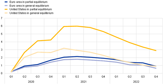
Source: ECB calculations.
Note: Simulations are based on Auclert et al., op. cit.
Further considerations reinforce the model-implied results of a moderate remaining additional boost to private consumption from excess savings, especially in the euro area. First, the different origin of the excess savings helps explain the smaller consumption impulse in the euro area compared with the United States. In the euro area, these excess savings were mostly due to mobility restrictions that limited consumption, especially for high-contact services, on which wealthy (low-MPC) households generally spend a larger share of their income. In the United States, the excess savings were mainly due to large stimulus packages that supported incomes, especially for (high-MPC) households at the bottom of the wealth distribution.[10] Second, recent price developments reinforce the view of a modest remaining consumption impulse from excess savings in both economies. Indeed, the rise in consumer prices and the decline in asset prices in recent quarters, amplified by the ongoing monetary policy tightening and deteriorating financing conditions, further reduce the remaining consumption impulse.
-
For related discussions see the boxes entitled “COVID-19 and the increase in household savings: precautionary or forced?”, Economic Bulletin, Issue 6, ECB, 2020; “COVID-19 and the increase in household savings: an update”, Economic Bulletin, Issue 5, ECB, 2021; “The implications of savings accumulated during the pandemic for the global economic outlook”, Economic Bulletin, Issue 5, ECB, 2021; “The recent drivers of household savings across the wealth distribution”, Economic Bulletin, Issue 3, ECB, 2022; and “Household saving during the COVID-19 pandemic and implications for the recovery of consumption”, Economic Bulletin, Issue 5, ECB, 2022. For an overview of the demand-side drivers of consumption, see the article entitled “The role of supply and demand in the post-pandemic recovery in the euro area” in this issue of the Economic Bulletin.
-
The stock of excess savings can be estimated as the cumulated difference between actual savings and their extrapolated pre-pandemic (2015-19) trend. The same methodology was applied to data for the United States by Aladangady, A., Cho, D., Feiveson, L. and Pinto, E., “Excess Savings during the COVID-19 Pandemic”, FEDS Notes, 21 October 2022. While the estimation of the stock of excess savings varies depending on the specific methodology used, the qualitative results comparing the euro area with the United States reported in this box do not change when alternative methods are used (for example, estimating the stock of excess savings as the cumulated difference between the current saving rate and its pre-pandemic level).
-
See Auclert, A., Rognlie, M. and Straub, L., “The Trickling Up of Excess Savings”, NBER Working Paper Series, No 30900, January 2023.
-
The preference of US households to hold their pandemic excess savings in liquid assets is corroborated by Abdelrahman H. and Oliveira L.E, “The Rise and Fall of Pandemic Excess Savings”, Economic Letter, FRBSF, 8 May 2023. Over the reference period, developments in loans to households may mask the effects of the US fiscal package (Coronavirus Aid, Relief, and Economic Security Act). This included forbearance of certain types of loan (student loans and certain mortgages), which lenders also offered for other loan types at their own volition. In addition, part of past-due loans were reclassified into forbearance, fictitiously increasing the flows of household loans. See Dettling, L. and Lambie-Hanson, L., “Why is the Default Rate So Low? How Economic Conditions and Public Policies Have Shaped Mortgage and Auto Delinquencies During the COVID-19 Pandemic”, FEDS Notes, 4 March 2021.
-
For the euro area, the distribution of excess savings across households is estimated using the ECB’s experimental Distributional Wealth Accounts, which combine quarterly developments in aggregate asset holdings with snapshots of household asset holdings in the Household Finance and Consumption Survey (HFCS). For the United States, it is estimated using the Federal Reserve Board Distributional Financial Accounts (DFA), which follow a similar methodology for aggregate asset holdings and household asset holdings in the Survey of Consumer Finances (SCF). The latest available data for the HFCS and the SCF refer to 2017 and 2019 respectively.
-
In the model, the sum of consumption for each household group is equal to aggregate demand and aggregate income.
-
Under general equilibrium, the model in this box considers the case of “rational expectations” described by Auclert et al., op. cit. In this case, households anticipate future changes in aggregate income.
-
As regards the MPC, recent empirical evidence finds that: (i) the average MPC has typically large values, and (ii) the share of holdings of liquid assets in household portfolios is a key driver of the considerable cross-sectional heterogeneity of the MPC. The specific values assumed in this box are taken from Slacalek, J., Tristani, O. and Violante, G., “Household balance sheet channels of monetary policy: A back of the envelope calculation for the euro area”, Journal of Economics Dynamics and Controls, Vol. 115, No 103879, June 2020. As regards the share of income, the values in this box are calibrated based on the 2017 HFCS for the euro area (entire distribution) and the 2019 SCF for the United States (median values).
-
See the speech by Philip Lane on “Inflation and monetary policy” given on 8 May 2023 and the box entitled “Inflation developments in the euro area and the United States”, Economic Bulletin, Issue 8, ECB, January 2023.
-
The US government paid a defined amount to citizens with an income of below USD 75,000. This implies that low-income citizens received a larger benefit in proportion to their income. See, for instance, the description of “Unemployment Compensation” and “Economic Impact Payments” provided by the U.S. Department of the Treasury.

